Carotid atherosclerotic plaque stability prediction from transversal ultrasound images using deep learning
Predikce stability aterosklerotického plátu z transverzálních ultrazvukových obrazů pomocí hlubokého učení
Cíl: Automaticky předpovídat stabilitu aterosklerotického plátu v karotidě ze standardních transverzálních ultrazvukových obrazů v B-modu za použití hlubokého učení. Spolehlivý prediktor by snížil potřebu klinických kontrol i farmakologické či chirurgické léčby. Metody: Automaticky byla lokalizována oblast zájmu obsahující karotidu. Adversariální metoda segmentace byla natrénována na kombinaci malého kompletně anotovaného datasetu a většího slabě anotovaného datasetu. Multikriteriální regrese s automatickou adaptací vah byla použita k predikci série klinicky relevantních atributů, vč. nárůstu tloušťky plátu během 3 let. Výsledky: Současnou šíři plátu bylo možno odhadnout s vysokou korelací (ρ = 0,32) a velmi vysokou statistickou signifikancí. Odhadovaný budoucí nárůst šíře plátu byl korelován méně (ρ = 0,22), ale stále statisticky významně (p < 0,01). Korelace mezi automatickým a expertním hodnocením echogenicity, hladkosti a kalcifikací byla ještě nižší. Závěr: Potvrdili jsme závislost mezi vzhledem plátu v ultrazvukovém obraze a pravděpodobností jeho budoucího růstu, ale je příliš slabá, než aby byla využitelná v klinické praxi jako jediný prediktor stability plátu.
Klíčová slova:
ateroskleróza – rizikový faktor – hluboké učení – ultrazvuk – progrese – karotida – zpracování biomedicínského obrazu – regresní analýza
Authors:
J. Kybic 1; D. Pakizer 2; J. Kozel 2; P. Michalčová 2; F. Charvát 3; D. Školoudík 3
Authors‘ workplace:
Faculty of Electrical Engineering, Czech Technical University in Prague, Czech Republic
1; Center for Health Research, Faculty of, Medicine, University of Ostrava, Czech, Republic
2; Central Military Hospital – Military, University Hospital, Prague, Czech, Republic
3
Published in:
Cesk Slov Neurol N 2024; 87(4): 255-263
Category:
Original Paper
doi:
https://doi.org/10.48095/cccsnn2024255
Overview
Aim: To automatically predict the stability of carotid artery plaque from standard B-mode transversal ultrasound images using deep learning. A reliable predictor would reduce the need for follow-up examination and pharmacological and surgical treatment. Methods: A region of interest containing the carotid artery was automatically localized. An adversarial segmentation method was trained on a combination of a small pixelwise annotated dataset and a larger weakly annotated dataset. A multicriterion regression with automatic weight adaptation was applied to predict a series of clinically relevant attributes, including the plaque width increase over 3 years. Results: The current plaque width could be estimated with a high correlation (ρ = 0.32) and a very high statistical significance. The estimated future increase of the plaque width was correlated less (ρ = 0.22) but statistically significantly (P < 0.01). The correlation between automatic and expert assessments of echogenicity, smoothness and calcification was even smaller. Conclusion: We confirmed a relationship between the plaque appearance in ultrasound and the probability of its future growth, but it is too weak to be used in clinical practice as the sole predictor of the plaque stability.
Keywords:
risk factor – deep learning – Regression analysis – ultrasound – Atherosclerosis – progression – carotid artery – biomedical image processing
Introduction
Carotid artery atherosclerotic plaques are present in over half of the population at the age of 50 [1]. In most cases, the plaques are stable, asymptomatic, and present no health hazard. However, some plaques keep growing rapidly and may lead to thrombosis or thromboembolism with possible blockage of the blood supply to the brain.
Atherosclerotic plaques can be studied by histology [2], CT, MRI [3], Doppler ultrasound [4] or other methods. Nowadays, the vast majority of carotid artery atherosclerotic plaques are detected by standard B-mode ultrasonographic screening [5]. This work aims to use these B-mode images to predict whether the plaque is stable (and will not grow substantially) or unstable and needs to be treated more aggressively. A success would have a profound effect in reducing the need for follow-up examinations, pharmacological treatment, and surgery.
Previous studies have shown that atherosclerotic plaque stability is related to some manually or semi-automatically evaluated characteristics derived from the ultrasound image such as the plaque width, surface irregularity and exulceration [6,7], echogenicity and homogeneity [8], neovascularity and complexity [9], or texture features [10]. However, the association found was weak, not allowing to make diagnostic decisions. More - over, there does not seem to be a consensus concerning relevant features. Some studies even found no significant relationship [11].
The goal of this work is to automatically predict the stability of carotid artery plaque from standard B-mode transversal ultrasound images using deep learning. We have previously shown a fully automatic image analysis pipeline [12] calculating geometry and wavelet features which were significantly different (p < 10–3) between stable and unstable plaques, but the accuracy of the predictor remained low (61–62%). Here we replace classical image analysis algorithms by deep learning methods, using several new techniques for this task, and hope to outperform the previous methods.
First, we employ adversarial learning techniques to learn to segment also from the electronic caliper images instead of only from full pixel-wise annotations. Second, we use multicriterion regression with automatic weight adjustment to predict not only the plaque width increase but also other parameters determined by the sonographers. We combine the segmentation mask and the original image as inputs to a relatively shallow multi-channel regression network. All techniques help to avoid overfitting and reduce the required annotation effort.
Materials and methods
Dataset
We used data from the clinical study ANTIQUE [13], from which we extracted images of 413 patients with a median age of 69 years who had an atherosclerotic plaque localized in the carotid bifurcation or proximal part of the internal carotid artery (ICA) with a width 2.0 mm or more and a degree of stenosis at least 30% in at least one examination. The patients were examined approximately every 6 months over the period of 3 years between 2015 and 2019 using Mindray DC8 ultrasound scanner (Mindray, Shenzhen, China) with a linear 3–12 MHz probe. All patients provided an informed consent and the images were anonymized before further processing. The images were categorized as transversal, longitudinal, conical and Doppler [12]. In this work, only transversal images were used. Two sets of images from two examination waves were analyzed for each patient – one immediately after enrollment and the second after 3 years.
Image attributes
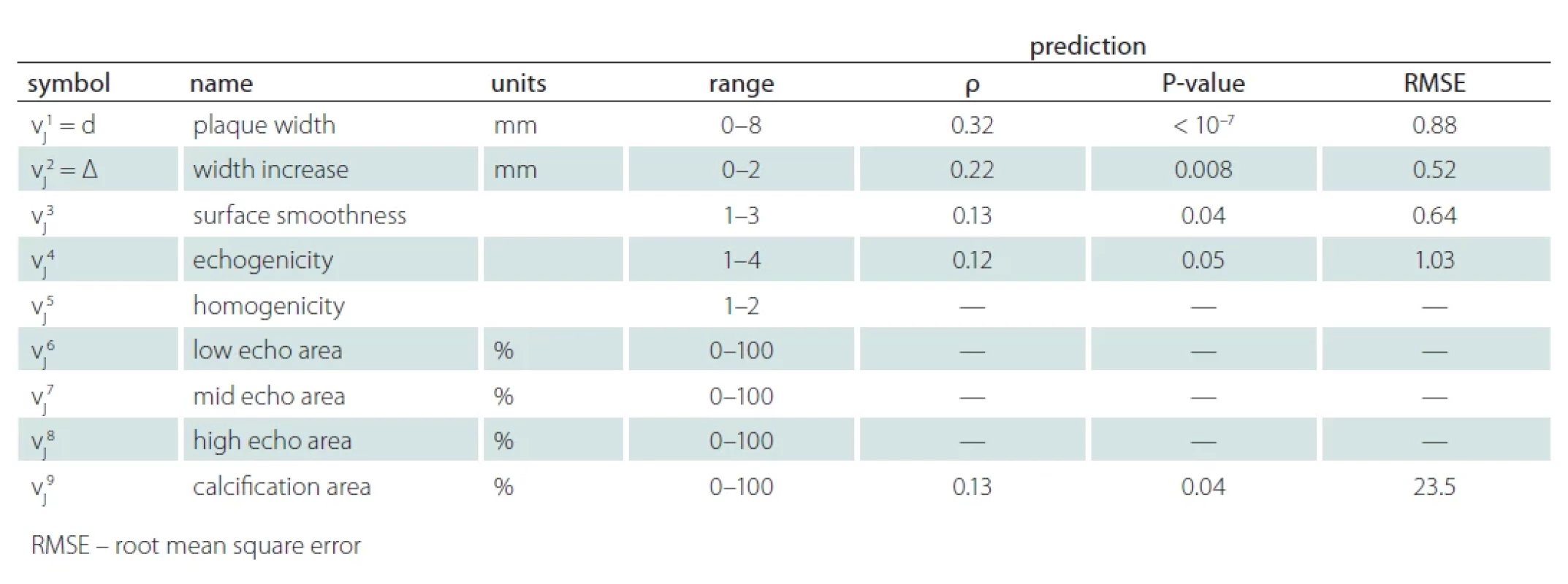
The experts used one key image to determine the plaque width (denoted d) in millimeters using virtual calipers as well as a set of image attributes describing the plaque appearance, such as echogenicity or homogeneity (see Tab. 1 for a full list). Our main prediction target was the positive part of the plaque width increase between the two examination waves:
D = max (d2 – d1, 0).
The full vector of the attributes for image j will be denoted vj = (vj1, vj2, …, vjA) with A = 9, vj1 = d being the plaque width and vj2 = D the width increase, etc.
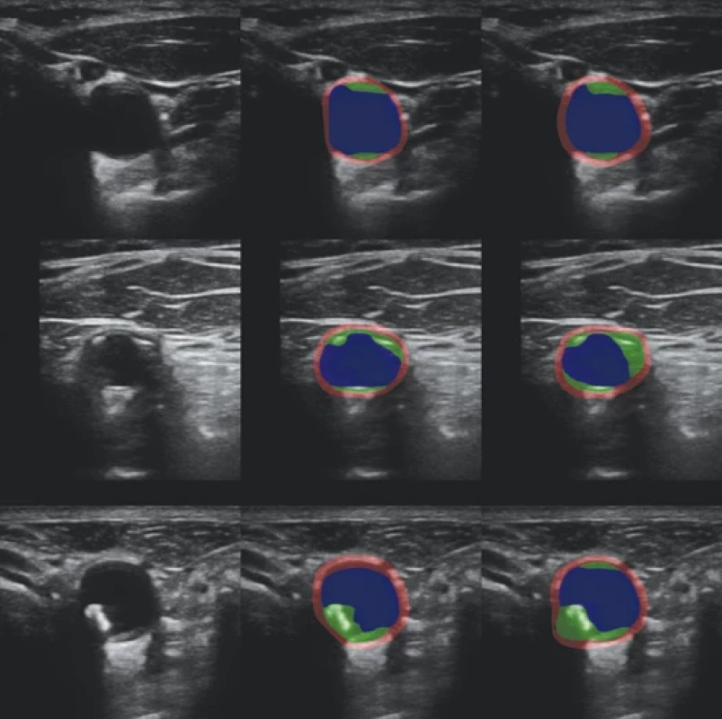
In this study, we only used key images to avoid discrepancies between the images and the expert annotations. For each patient and each side (left and right), we therefore had two images, called first and second. See Fig. 1 (left) for an example.
Localization
For each transversal image, the lumen of the ICA was automatically localized using a Faster R-CNN architecture [14] trained on 300 manually annotated images, as described in [12]. A region of interest (ROI) centered over the carotid artery of size 520 × 520 pixels was extracted. See Fig. 1 (center) and 2 (left) for examples.
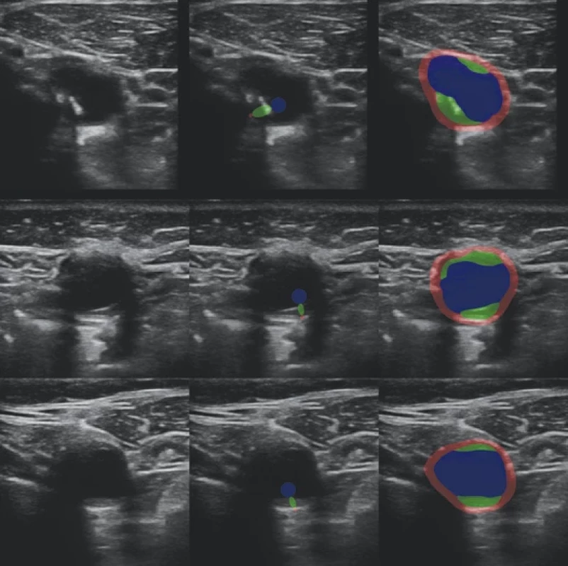
For each key image, an image with the distance markers (virtual calipers) in green was available (Fig. 1). The cross marker is located at the interface between the plaque and the lumen and a dashed line connects it with the vessel wall. We located the cross by template matching in the green channel and the wall interface point was determined as the furthest green point from the marker. Note that markers were not used for the ROI localization or any other processing, so our method is not restricted to key images.
From the 413 × 2 × 2 = 1,652 potential key images, 1,399 were available after ROI and marker localization described above. These were randomly split into training (80%) and testing (20%) part, yielding 568 training and 147 testing images to estimate D (from the first examination wave only) and 1 113 training and 286 testing images to estimate the plaque width d and all other attributes (from both examination waves).

Segmentation
To train the segmentation network, we used two sets of annotations, strong and weak. In the smaller, strongly annotated dataset Ωs, experts assigned each pixel to one of m = 4 classes (1 – background, 2 – vessel wall, 3 – plaque, and 4 – lumen) [12], see Fig. 2. There were 111 training (80%) and 27 testing images (20%), distinct from the key images described above. To increase the segmentation dataset size, we leveraged the already identified distance markers. We put an ellipsoidal mask with an aspect ratio 1 : 4 for the plaque class over the line connecting the two markers and circular masks with the radii 20 and 5 pixels touching the line from the outside for the lumen and wall classes, respectively (see Fig. 3, right). This way, we obtained weak segmentation annotations for all 1,399 key images without requiring any additional time-consuming manual annotation. We denoted the dataset Ωw. The annotations are called weak because only a small part of the pixels is annotated, which can nevertheless guide the segmentation to the correct location of the plaque. Both strong and weak annotations can be represented by one-hot encoding, using an indicator vector yi = (yi1, yi2, yi3, yi4) Î {0,1} m for each pixel i, with yi1=1 indicating background, yi2 = 1 the vessel wall etc. For strong annotations the class is always determined, ∑kyik = 1, while for weak annotations in undetermined pixels yi = (0,0,0,0).
The segmentation convolutional neural network (CNN) S uses a standard U-net [15] architecture with Resnet34 [16] backbone and softmax output layer with an m = 4 channel output f in the range [0,1]. The network was trained on a union Ω = Ωs È Ωw of strongly and weekly annotated datasets, minimizing the cross-entropy segmentation loss function
where the indices j, i, k correspond to training images, pixels and classes, respectively. This way, the undetermined pixels in the weakly annotated images are automatically ignored. The strongly annotated dataset is oversampled 15× to give it more weight. To combat overfitting, we used a wide range of augmentation operations: random horizontal flipping, small translations, rotations and scaling changes, changes of brightness and contrast, and multiplicative and additive noise.
Adding the weakly annotated dataset improves the segmentation results with respect to using only the small strongly annotated dataset [12]. However, we found that the U-net nevertheless sometimes produced unrealistic and physiologically unfeasible segmentations. As a remedy, we used generative adversarial nets (GANs) [17] to learn the model of likely segmentations [18]. Besides the segmentation network S, we therefore also trained a discriminator D, which should learn to distinguish ‘real’ human expert segmentations from the strongly annotated dataset on one side, from ‘fake’ segmentations produced by S on both strongly and weakly annotated images on the other side. The segmentation network S then learns to generate plausible segmentations which are accepted by the discriminator D as “real”.
We trained the segmentation network S to minimize the combined loss function
which rewards S for generating segmentations that are evaluated by the discriminator D as “real”, corresponding to D (S (xi)) ≈ 1. The coefficient a controls the trade-off between the segmentation error and the prior. We used a = 100, the exact value does not seem to be critical.
In contrast, the discriminator D was trained to minimize
encouraging D to classify all expert segmentations from Ωs as ‘real’ (D ≈ 1) and all segmentations generated by S (from both Ωs and Ωw) as ‘fake’ (D ≈ 0).
It is notoriously difficult to prevent the discriminator D to work too well and thus deprive the segmentor from useful gradient feedback, especially in the beginning, when S is not well trained. To make the task more difficult for the discriminator, we used three strategies. First, we added label noise (randomly flipping the real/fake label with probability 0.1) and we also degraded the segmentations by adding a uniform noise with amplitude 0.3 to the class probabilities yj and S (xj) and blurring them with a Gaussian filter with σ = 3 „pixels“. The probabilities were renormalized to sum to unity afterwards. Second, we switched between optimizing S and D based on the performance of the discriminator D. When its accuracy in distinguishing ‘real’ from ‘fake’ segmentations exceeded 60%, we switched to optimizing the segmentor S. When the accuracy dropped below 40%, we stoped optimizing S and started optimizing D. We used the Adam optimizer with a relatively small step size 10–5.
Third, the discriminator CNN D is very small. It is a simplified version of the discriminator network from [19], using 4 convolutional layers with 3 × 3 kernels and 16, 32, 64 and 128 channels, respectively. We used leakyReLU non-linearities, dropout (with probability 0.25), and instance normalization after every convolutional layer. The final linear layer with sigmoid nonlinearity produces the desired output value D (y) Î [0,1].
Examples of automatic segmentations are shown in Fig. 2 and 3 (right column) for the strongly and weekly annotated images, respectively.
segmentace.
automatická plná segmentace.
Regression
The image attributes vj to be predicted are linearly normalized to the range [0,1] (see Table 1 for the original ranges) for better numerical stability. We chose to minimize a weighted mean squared error (MSE):
where v˜ji = (v˜j1… v˜jA) are the normalized expert-determined attributes, vˆji = (vˆj1 … vˆjA) = R (uj) are the normalized predictions and R is the prediction network with input uj associated with image j (see below for details).

The benefits of this multicriterion optimization are twofold. First, automatically predicting these plaque image attributes is useful in its own right, as they appear to be clinically relevant [6]. Second, learning multiple objectives from a shared representation is known to improve the learning efficiency and prediction accuracy [20], probably by making it more difficult to overfit. However, the benefit depends on the appropriate choice of the weights wi, which are difficult and time consuming to tune manually. Fortunatelly, a maximum likelihood formulation with a Gaussian model suggested in [20] allows us to treat the weights wi = 1/ (2σi2) as additional parameters of a modified loss function
This way, an equilibrium is found so that well estimated attributes are given more weight. We also get an estimate σi2 of the estimation error. For numerical reasons, we optimize zi = log wi instead of wi directly.
We used a small shallow CNN [21] as the regression network R, so that it is less prone to overfitting and concentrates on texture rather than shape. It consists of 5 convolutional layers with 3 × 3 kernels, with 32, 64,128,256, and 64 channels, respectively, each followed by batch normalization, max-pooling, ReLU nonlinearity, and dropout. At the end, the number of channels was reduced to A and passed again through batch normalization, ReLU nonlinearity, dropout, and a final linear layer.
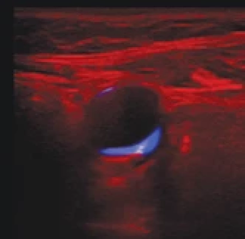
The usual approach would be to feed the regression network R the input image multiplied by a mask, leaving only the plaque region. This would allow the regression network to focus on the plaque region. Some features, like the plaque width, can be directly derived from the plaque mask. Unfortunately, this makes the regression vulnerable to segmentation errors. Alternatively, we could use the original, unmasked images as inputs, thus avoiding the dependency on the segmentation. Unfortunately, our set of image annotations was too small to train the regression network to focus on the plaque. We therefore decided to combine these approaches and use three channels as the input u = (u1, u2, u3) of the regression network R. The first channel is the cropped grayscale image
ui1 = xi
the second is the image limited to the plaque region using the automatic segmentation output
ui2 = xi [argmax fik = 3]
k
where [·] is the Iverson bracket, equal to 1 if the expression is true and 0 otherwise. The third channel is the (soft) plaque mask itself
ui3 = fi3
where i is the pixel index, f is the segmentation network output and 3 corresponds to the plaque class. See Fig. 4 for an example.
To encourage the network to use all channels, we randomly replaced each channel with zeros with the probability 0.5. This can be considered a channel-level dropout. Other augmentation operations were standard: random horizontal flip, rotation ± 40°, scale change ± 10%, and random cropping to the final input size 384 × 384 pixels.
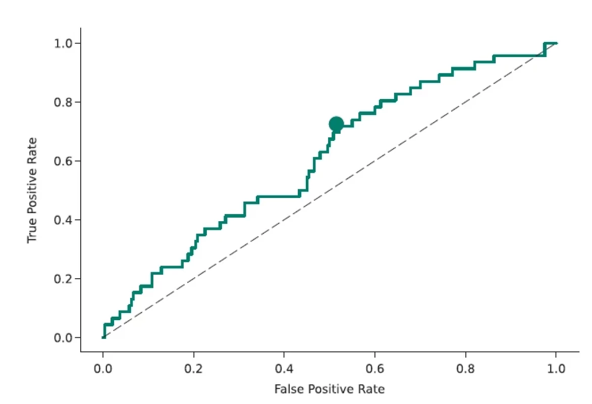
Obr. 6. ROC křivka klasifi kátoru rozlišujícího mezi stabilními a progresivními pláty, definovaná jako Δ ≥ 0,4 mm. Tečka odpovídá pracovnímu bodu maximalizujícímu hodnotu F1. Přerušovaná čára odpovídá náhodnému výběru. AUC = 0,609.
AUC – plocha pod křivkou; ROC – receiver operating characteristic
Results
The prediction performance was evaluated on the test part of the dataset (not used in training) by comparing the predicted and reference (expert-determined) attributes vji. Table 1 shows the calculated root mean squared error (RMSE, after denormalization to the original range), the Pearson’s correlation coefficient ρ and the associated probability P (significance) of an uncorrelated system producing |ρ‘|>|ρ| under the normality assumption (calculated using the Pearson´s function from the SciPy Python library). We do not show these performance criteria if the correlation is not significant at least at the 0.05 level.
We see that out of the 9 image attributes, we can predict two at the 0.01 significance level. First, the estimation of the plaque width d correlates very significantly with the reference values, although the ρ = 0.32 correlation is far from the ideal value of ρ = 1. Second, our estimate of D, the future increase of the plaque width, is also significantly correlated with the reference values, although the correlation is smaller, ρ = 0.22. Fig. 5 shows the predicted and reference values as a scatter plot. We can see that the correlation is indeed present but weak. Note also that the distribution of D is highly non-symmetric – low values of D are much more frequent than high values, making the regression challenging.
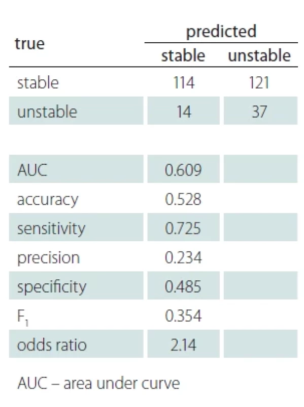
Besides regression, we also evaluated the prediction of D in a binary classification problem framework. The two classes are stable and unstable, defined by thresholding D ≥ t. For comparability with [6,12], the threshold was set at t = 0.4 mm, which corresponds to twice the estimated plaque width measurement error. Fig. 6 shows the ROC (receiver operating characteristic curve) of this classifier with a working point maximizing the F1 score. The confusion matrix and standard binary classification performance measures are shown in Tab. 2. We see that the classifier is far from perfect, but also clearly above random choice.
Discussion and conclusions
Using artificial intelligence methods for carotid plaque detection and characterization in ultrasound, as well as in other modalities, is an active area of research described in a number of review articles [22,23]. However, most of these works aimed to characterize the current state. As an example, there is a CAD (computer aided diagnostic) system [24] capable of differentiating between symptomatic and asymptomatic plaques with nearly perfect AUC = 0.956 (area under the ROC curve), with some manual steps. In that case, however, symptomatic plaque means that the patient is currently experiencing stroke, transient ischemic attack (TIA), or amaurosis fugax (AF, transient loss of vision). This is very different from the prediction task we are solving, which aims to predict future state, in order to be able to take preventive measures in time to avoid serious complications such as a stroke.
The gold standard in carotid plaque imaging is now MRI [3], with ultrasound providing much less information. A number of image features seem to be statistically relevant for distinguishing symptomatic plaques [9] but much less so for the prediction [6]. Contrast ultrasound was found not to be useful to identify vulnerable plaques in asymptomatic patients [11], which gives even less hope to non-contrast ultrasound.
Histology classification after endarterectomy was found to correlate with plaque being symptomatic [2]. There were therefore attempts to correlate the ultrasound image features with information from histology. However, the reported AUC = 0.68 (95% confidence interval 0.59–0.78) [7] is not significantly better than ours (0.609).
It can therefore be expected that predicting future plaque growth from ultrasound is difficult. Our achieved performance indicators on this task are modest but appear to be comparable to previously reported results. For example, our AUC = 0.609 (Tab. 2) is almost identical to AUC = 0.604 in [12]. Our odds ratio OR = 2.14 is very much comparable to the highest reported OR = 2.328 (for ulcerated surface, confidence interval 1.42–3.82) in [6] and higher than all others. Let us also emphasize our relatively good performance in determining the current plaque width, which we already know to be a relevant factor for predicting the stability [6].
Since our deep-learning created features are not directly related to human-designed features used before [12], there is a hope that combining them might further improve the prediction performance. On the other hand, a pessimistic interpretation of our results is that further improvement is unlikely since the plaque growth depends on other factors that are not captured by the ultrasound image.
We yet need to explain our failure to predict the other image attributes, such as echogenicity and homogeneity. We can only hypothesize that this might be caused by inconsistent annotations, as characterizing plaques with a naked eye is often unreliable and has high intra - and inter-observer variability [22,25].
From the methodological point of view, we have applied several new techniques to both segmentation and regression, which might be useful for other tasks, too. They are based on previous work but adapted to our task. In particular, we have used GANs to model feasible segmentations, employed automatically generated weak annotations, and multi-criterion and multi-channel regression with channel-level dropout.
Ethics approval
The study was performed according to Helsinki Declaration of 1975 (and its 2004 and 2008 revisions). All participants provided an informed consent. We used data from the clinical study ANTIQUE [13], which was approved by the Ethics Board of the Faculty Hospital Ostrava (approval number 605/2014, 31 July 2014) and Ethics Committee of the Central Military Hospital Prague (approval number 108/12-44/2018, 11 June 2018). All participants provided an informed consent.
Funding
The authors acknowledge the support of the Czech Health Research Council project NV19-08-00362. All rights reserved.
Competing interests
The authors have no relevant financial or non-financial interests to disclose.
Author Contributions
Jan Kybic performed image analysis, machine learning, implementation, experiments, writing and editing. David Pakizer, Jiří Kozel and Patricie Michalčová performed data annotation. František Charvát performed data collection and evaluation. David Školoudík suggested the concept, provided medical expertise, and worked on data acquisition, curation, and editing. All authors read and approved the final manuscript.
Consent to publish
This manuscript contains no identifiable individual’s personal data.
Acknowledgements
We thank M. Hekrdla for data curation, M. Kostelanský, D. Baručić, A. Manzano-Rodriguez, and S. Kaushik for implementing and making available the method described in [12], and O. Dvorský for setting up the CVAT annotation server.
Sources
1. Salonen R, Seppänen K, Rauramaa R et al. Prevalence of carotid atherosclerosis and serum cholesterol levels in eastern Finland. Arteriosclerosis 1988; 8 (6): 788–792. doi: 10.1161/01.atv.8.6.788.
2. Svoboda N, Voldřich R, Mandys V et al. Histological analysis of carotid plaques: the predictors of stroke risk. J Stroke Cerebrovasc Dis 2022; 31 (3): 106262. doi: 10.1016/j.jstrokecerebrovasdis.2021.106262.
3. Brinjikji W, Huston J, Rabinstein AA et al. Contemporary carotid imaging: from degree of stenosis to plaque vulnerability. J Neurosurg 2016; 124 (1): 27–42. doi: 10.3171/2015.1.JNS142452.
4. Chen X, Kong Z, Wei S et al. Ultrasound lmaging-vulnerable plaque diagnostics: automatic carotid plaque segmentation based on deep learning. J Radiat Res 2023; 16 (3): 100598. doi: 10.1016/j.jrras.2023.100598.
5. Nicolaides A, Beach KW, Kyriacou E et al. Ultrasound and carotid bifurcation atherosclerosis. London: Springer-Verlag 2013. doi: 10.1007/978-1-84882-688-5.
6. Školoudík D, Kešnerová B, Hrbáč T et al. Vizuální hodnocení a digitální analýza ultrazvukového obrazu u stabilního a progredujícího aterosklerotického plátu v karotické tepně. Cesk Slov Neurol N 2021; 84/117 (1): 38–44. doi: 10.48095/cccsnn202138.
7. Salem MK, Bown MJ, Sayers RD et al. Identification of patients with a histologically unstable carotid plaque using ultrasonic plaque image analysis. Eur J Vasc Endovasc Surg 2014; 48 (2): 118–125. doi: 10.1016/j.ejvs.2014. 05.015.
8. Doonan RJ, Gorgui J, Veinot JP et al. Plaque echodensity and textural features are associated with histologic carotid plaque instability. J Vasc Surg 2016; 64 (3): 671–677.e8. doi: 10.1016/j.jvs.2016.03.423.
9. Brinjikji W, Rabinstein AA, Lanzino G et al. Ultrasound characteristics of symptomatic carotid plaques: a systematic review and meta-analysis. Cerebrovasc Dis 2015; 40 (3–4): 165–174. doi: 10.1159/000437339.
10. Kakkos SK, Nicolaides AN, Kyriacou E et al. Computerized texture analysis of carotid plaque ultrasonic images can identify unstable plaques associated with ipsilateral neurological symptoms. Angiology 2011; 62 (4): 317–328. doi: 10.1177/0003319710384397.
11. D‘Oria M, Chiarandini S, Pipitone MD et al. Contrast Enhanced Ultrasound (CEUS) is not able to identify vulnerable plaques in asymptomatic carotid atherosclerotic disease. Eur J Vasc Endovasc Surg 2018; 56 (5): 632–642. doi: 10.1016/j.ejvs.2018.07.024.
12. Kostelanský M, Manzano-Rodríguez A, Kybic J et al. Differentiating between stable and progressive carotid atherosclerotic plaques from in-vivo ultrasound images using texture descriptors. In: Proceedings of the SPIE 2021; 12088 : 120881L 10. doi: 10.1117/12.2605 795.
13. Školoudík D. Atherosclerotic plaque characteristics associated with a progression rate of the plaque in carotids and a risk of stroke. Clinical trial NCT02360137 (2015). [online]. Available from: https: //clinicaltrials.gov/ct2/ show/NCT02360137.
14. Ren S, He K, Girshick RB et al. Faster R-CNN: Towards real-time object detection with region proposal networks. IEEE Trans Pattern Anal Mach Intell 2017; 39 (6): 1137–1149. doi: 10.1109/TPAMI.2016.2577031.
15. Ronneberger O, Fischer P, Brox T. U-Net: convolutional networks for biomedical image segmentation. In: Navab N, Hornegger J, Wells W et al. (eds). Medical Image Computing and Computer-Assisted Intervention – MICCAI 2015. Lecture Notes in Computer Science (LNIP). Freiburg: Springer 2015.
16. He K, Zhang X, Ren S et al. Deep Residual learning for image recognition. In: Proceedings of 2016 IEEE Conference on Computer Vision and Pattern Recognition (CVPR). Las Vegas: IEEE Xplore 2016 : 770–778. doi: 10.1109/CVPR.2016.90.
17. Goodfellow I, Pouget-Abadie J, Mirza M et al. Generative adversarial nets. In: Ghahramani Z, Welling M, Cortes C et al. (eds). Advances in neural information processing systems, vol. 27. San Francisco: Curran Associates, Inc. 2014.
18. Valvano G, Leo A, Tsaftaris SA. Learning to Segment from scribbles using multi-scale adversarial attention gates. IEEE Trans Med Imaging 2021; 40 (8): 1990–2001. doi: 10.1109/TMI.2021.3069634.
19. Mao X, Li Q, Xie H et al. Least squares generative adversarial networks. In: Proceedings of 2017 IEEE International Conference on Computer Vision (ICCV). Venice: IEEE Xplore 2017 : 2813–2821. doi: 10.1109/ICCV. 2017.304.
20. Cipolla R, Gal Y, Kendall A. Multi-task learning using uncertainty to weigh losses for scene geometry and semantics. In: Proceedings of 2018 IEEE/CVF Conference on Computer Vision and Pattern Recognition (CVPR). Salt Lake City: IEEE Xplore 2018 : 7482–7491. doi: 10.1109/CVPR.2018.00781.
21. Peng H, Gong W, Beckmann CF et al. Accurate brain age prediction with lightweight deep neural networks. Med Image Anal 2021; 68 : 101871. doi: 10.1016/j.media.2020.101871.
22. Saba L, Sanagala SS, Gupta SK et al. Multimodality carotid plaque tissue characterization and classification in the artificial intelligence paradigm: a narrative review for stroke application. Ann Transl Med 2021; 9 (14): 1206. doi: 10.21037/atm-20-7676.
23. Miceli G, Rizzo G, Basso MG et al. Artificial intelligence in symptomatic carotid plaque detection: a narrative review. Applied Sciences 2023; 13 (7): 4321. doi: 10.3390/ app13074321.
24. Skandha SS, Gupta SK, Saba L et al. 3-D optimized classification and characterization artificial intelligence paradigm for cardiovascular/stroke risk stratification using carotid ultrasound based delineated plaque: Atheromatic™ 2.0. Comput Biol Med 2020; 125 : 103958. doi: 10.1016/j.compbiomed.2020.103958.
25. Svoboda N, Bradac O, Mandys V et al. Diagnostic accuracy of DSA in carotid artery stenosis: a comparison between stenosis measured on carotid endarterectomy specimens and DSA in 644 cases. Acta Neurochir (Wien) 2022; 164 (12): 3197–3202. doi: 10.1007/s00701-022-053 32-5.
Labels
Paediatric neurology Neurosurgery NeurologyArticle was published in
Czech and Slovak Neurology and Neurosurgery

2024 Issue 4
-
All articles in this issue
- Editorial
- The Trail Walking Test to predict probable mild cognitive impairment in older adults
- Physical activity in people with multiple sclerosis and the impact of the COVID-19 pandemic
- Carotid atherosclerotic plaque stability prediction from transversal ultrasound images using deep learning
- Influencing factors for axial symptoms after modified expansive open-door laminoplasty
- Association between surgical results and recurrence in benign and intermediate osteogenic spine tumors – osteoid osteomas and osteoblastomas
- Development of cognitive performance in children before and after surgical treatment of pharmacoresistant temporal lobe epilepsy
- Cutaneous ischemia and vertebral body infarction indicating spinal cord ischemia
- Poděkování zakládajícím členům SOR
- Myastenie gravis – jak léčit pacienty co nejefektivněji?
- Abstrakta z XII. neuromuskulárního kongresu 18.– 19. 4. 2024 v Brně
- Czech and Slovak Neurology and Neurosurgery
- Journal archive
- Current issue
- About the journal
Most read in this issue
- The Trail Walking Test to predict probable mild cognitive impairment in older adults
- Myastenie gravis – jak léčit pacienty co nejefektivněji?
- Physical activity in people with multiple sclerosis and the impact of the COVID-19 pandemic
- Development of cognitive performance in children before and after surgical treatment of pharmacoresistant temporal lobe epilepsy


